Machine Learning Revision
Table of Contents
1 About This Document
This document contains my revision notes for COMP3206 Machine Learning as taught by Professor Mahesan Niranjan at the University of Southampton. This work was produced based on his lectures but any inaccuracies and misunderstandings contained herein are almost certainly my own mistake. This does not represent the whole module, only what I expect to find on the exam.
This document may be distributed under the terms of the GNU Free Documentation Licence. A copy of the licence can be found here. Please feel free to ask questions and contribute improvements at the git repo.
2 Maths Review
This section very briefly reviews some of the maths needed for the rest of the document.
2.1 Matrices and Vectors
2.1.1 Basics
A vector:
\begin{equation*} \mathbf{x} = \begin{pmatrix} x_1 \\ x_2 \\ x_3 \\ \vdots \\ x_N \end{pmatrix} \end{equation*}A matrix:
\begin{equation*} \mathbf{A} = \begin{pmatrix} a_{11} & a_{12} & \cdots & a_{1n} \\ a_{21} & a_{22} & \cdots & a_{2n} \\ \vdots & \vdots & \vdots & \vdots \\ a_{m1} & a_{m2} & \cdots & a_{mn} \\ \end{pmatrix} \end{equation*}Matrix Multiplication:
\begin{equation*} [\mathbf{A}\mathbf{B}]_{ij} = \sum_{k=1}^n A_{ik}B_{kj} \end{equation*}Scalar product of vectors: (where θ is the angle between the vectors)
\begin{equation*} \mathbf{x} \cdot \mathbf{y} = \sum_{i = 1}^{N} x_i y_i = \mathbf{x}^T \mathbf{y} = |\mathbf{x}| |\mathbf{y}| \cos(\theta) \end{equation*}This can be used to project \(\mathbf{x}\) along the direction \(\mathbf{u}\):
\begin{equation*} \mathrm{projection} = \frac{\mathbf{x}^T \mathbf{u}}{|\mathbf{u}|}\mathbf{u} \end{equation*}As an example of matrix algebra: a diagonal matrix is a scalar multiple of the identity matrix. A diagonalizable matrix can be written in terms of a diagonal matrix \(\mathbf{D}\) and some transformation matrix \(\mathbf{S}\) as follows:
\begin{equation*} \mathbf{A} = \mathbf{SDS}^{-1} = \mathbf{S}a\mathbf{IS}^{-1} \end{equation*}Using this relationship, a diagonalizable matrix can be efficiently raised to a power using
\begin{equation*} \mathbf{A}^n = \mathbf{SD}^n\mathbf{S}^{-1} = \mathbf{S}a^n\mathbf{IS}^{-1} \end{equation*}To prove this by induction for \(n \in \mathbb{N}\):
\begin{align*} \mathbf{A}^1 =& \mathbf{SD}^1\mathbf{S}^{-1} \\ \mathrm{Assume } \: \mathbf{A}^n =& \mathbf{SD}^n\mathbf{S}^{-1} \\ \mathbf{A}^{n+1} = \mathbf{A}^n\mathbf{A} =& \mathbf{SD}^n\mathbf{S}^{-1}\mathbf{SD}\mathbf{S}^{-1} \\ =& \mathbf{SD}^n\mathbf{D}\mathbf{S}^{-1} \\ =& \mathbf{SD}^{n+1}\mathbf{S}^{-1} \\ \end{align*}2.1.2 Linear Transformation
Following from the definition of matrix multiplication, linear transformations on vectors can be represented using a matrix. For example, a vector \(\mathbf{x} \in \mathbb{R}^2\) can be rotated by θ by multiplying with a matrix to give a new vector \(\mathbf{r} \in \mathbb{R}^2\).
\begin{equation*} \mathbf{r} = \begin{pmatrix} \cos(\theta) & -\sin(\theta) \\ \sin(\theta) & \cos(\theta) \\ \end{pmatrix} \mathbf{x} \end{equation*} \begin{equation*} |\mathbf{x}| = |\mathbf{r}| \end{equation*}A special case of these linear transformations is to only scale the vector by some amount \(\lambda\):
\begin{equation*} \mathbf{Ax} = \lambda \mathbf{x} \end{equation*}For a matrix \(\mathbf{A}\), the vectors \(\mathbf{x}\) and scalars \(\lambda\) which satisfy this equation are called eigen vectors and eigen values, respectively. They can be found by the following method:
\begin{align*} \mathbf{Ax} =& \lambda \mathbf{x} \\ \mathbf{Ax} - \lambda \mathbf{x} =& 0 \\ (\mathbf{A} - \lambda\mathbf{I})\mathbf{x} =& 0 \end{align*}For non-trivial results:
\begin{align*} \mathrm{det}(\mathbf{A} - \lambda\mathbf{I}) = 0 \end{align*}As another example of a linear transformation, take a vector \(\mathbf{u} \in \mathbb{R}^d\) and from it construct the matrix \(\mathbf{P} = \mathbf{uu}^T\). The first interesting property of this matrix is that multiplying it with any vector will make a vector which points in the direction of \(\mathbf{u}\):
\begin{align*} \mathbf{Px} = \mathbf{uu}^T\mathbf{x} = \mathbf{u}(\mathbf{u}\cdot\mathbf{x}) = \mathbf{u}a \end{align*}This works because the dot product results in a scalar (written as \(a\)).
Another use for \(\mathbf{P}\) is to construct \((2\mathbf{P} - \mathbf{I})\), which will reflect around \(\mathbf{u}\):
\begin{align*} (2\mathbf{P} - \mathbf{I})\mathbf{x} &= 2\mathbf{Px} - \mathbf{x} \\ &= 2\mathbf{u}(\mathbf{u}\cdot\mathbf{x}) - \mathbf{x} \end{align*}To see this, it helps to sketch it.
2.2 Calculus
2.2.1 Basics
For a function \(f\: : \: \mathbb{R}^N \to \mathbb{R}\)
\begin{equation*} \mathbf{\nabla f} (\mathbf{x}) = \begin{pmatrix} \frac{\partial f}{\partial x_1} \\ \frac{\partial f}{\partial x_2} \\ \vdots \\ \frac{\partial f}{\partial x_N} \\ \end{pmatrix} \end{equation*}\(\mathbf{\nabla f}\) should be thought of as the vector gradient of \(f\).
For example, consider \(f(\mathbf{x}) := \mathbf{x}^T\mathbf{Ax}\), \(\mathbf{x} \in \mathbb{R}^2\), where \(\mathbf{A}\) is symmetric (\(A_{21} = A_{12}\))
\begin{align*} \mathbf{\nabla f} &= \begin{pmatrix} \frac{\partial f}{\partial x_1}\left( x_1^2A_{11} + 2x_1x_2A_{21} + x_2^2A_{22} \right) \\ \frac{\partial f}{\partial x_2}\left( x_1^2A_{11} + 2x_1x_2A_{21} + x_2^2A_{22} \right) \\ \end{pmatrix} \\ &= \begin{pmatrix} 2x_1A_{11} + 2x_2A_{21} \\ 2x_2A_{22} + 2x_1A_{21} \\ \end{pmatrix} \\ &= 2\mathbf{Ax} \end{align*}Usually I will write this as \(\partial f/\partial \mathbf{x}\) so as to distinguish this from the case where \(f\) is a function of several vectors (for which I will use \(\mathbf{\nabla}\)).
Similarly, \(\mathbf{H}\) (the hessian matrix). This represents the local curvature of a function \(f\: : \: \mathbb{R}^N \to \mathbb{R}\) using second order partial derivatives. The hessian matrix can be defined as
\begin{equation*} H_{ij} = \frac{\partial^2 f}{\partial x_i \partial x_j} \end{equation*}2.2.2 Optimisation
- Unconstrained
For example \(\min f(\cdot)\)
A commonly used iterative method is gradient decent:
\begin{equation*} \mathbf{x}^{(n+1)} = \mathbf{x}^{(n)} - \eta \mathbf{\nabla f(\mathbf{x})} \end{equation*}Gradient decent is like taking the path down the gradient to the bottom of the metaphorical hill.
Newton's method converges faster than gradient decent but is also far more computationally intensive
\begin{equation*} \mathbf{x}^{(n+1)} = \mathbf{x}^{(n)} - \eta\mathbf{H}^{-1}\mathbf{f(\mathbf{x})} \end{equation*} - Constrained - Lagrange Multipliers
To minimise \(f \: : \: \mathbb{R}^n \to \mathbb{R}\) subject to conditions \(g_i \: : \mathbb{R}^{d_i} \to \mathbb{R} = 0, \: d_i\leq n, \: i = 1, 2, \dots, m\), define \(\mathcal{L} \: : \: \mathbb{R}^{n+m} \to \mathbb{R} \: := f(\cdot) - \sum_{i=1}^{N}\lambda_i g_i(\cdot)\). The minimum (or maximum) will be at \(\mathbf{\nabla \mathcal{L}} = \mathbf{0}\).
Example: Minimise \(f(x,y)=xy\) subject to \(x^2+y^2=8\)
\begin{align*} &g(x,y) = x^2+y^2-8 \\ &\mathcal{L}(x,y,\lambda) = xy - \lambda(x^2+y^2-8) \\ &\mathbf{\nabla \mathcal{L}}(x,y,\lambda) = \mathbf{0} \\ &\frac{\partial \mathcal{L}}{\partial x} = y - 2\lambda x = 0 \\ &\frac{\partial \mathcal{L}}{\partial y} = x - 2\lambda y = 0 \\ &\therefore x = y \\ &\frac{\partial \mathcal{L}}{\partial \lambda} = x^2 + y^2 -8 = 0 \\ &\therefore 2x^2 - 8 = 0 \\ &\therefore x = y = \pm 2 \end{align*}So there are minima subject to the constraint at \((2,2)\) and \((-2, -2)\).
2.3 Probability
2.3.1 Bayes Theorem
For \(N\) classes
\begin{equation*} P[Y|X] = \frac{P[X|Y]P[Y]}{\sum_{i=1}^{N} P[X|Y_i] P[Y_i]} \end{equation*}2.3.2 Multivariate Gaussian
For a mean \(\mathbf{m} \in \mathbb{R}^p\) and co-variance matrix \(\mathbf{C} \in \mathbb{R}^{p \times p}\)
\begin{equation*} p(\mathbf{x}) = \frac{1}{\sqrt{(2\pi)^p \mathrm{det}(\mathbf{C})}}\exp\left(-\frac{1}{2}(\mathbf{x} - \mathbf{m})^T\mathbf{C}^{-1}(\mathbf{x} - \mathbf{m})\right) \end{equation*}The normal (gaussian) distribution can be linearly transformed as so:
\begin{align*} \mathbf{x} \sim& \mathcal{N}(\mathbf{m}, \mathbf{C}) \\ \mathbf{Ax} \sim& \mathcal{N}(\mathbf{Am}, \mathbf{ACA}^T) \end{align*}3 Supervised Learning
3.1 Function Approximation
3.1.1 Linear Regression
Multivariate linear regression is concerned with learning a function \(f \: : \: \mathbb{R}^p \to \mathbb{R}\) such that the function predicts some useful variable from the inputs. For example, predicting housing prices from the size of the house and it's distance from a school.
In linear regression we use a function of the form
\begin{equation*} f(\mathbf{x}) := \mathbf{w}^T\mathbf{x} + w_0 \end{equation*}For convenience we will work in \(p+1\) dimensional space:
\begin{align*} &\mathbf{y} = (\mathbf{x} \quad 1)^T \\ &\mathbf{a} = (\mathbf{w} \quad w_0)^T \\ &f = \mathbf{y}^T\mathbf{a} \\ \end{align*}The function \(f\) forms our model, we have some training data \(\{\mathbf{y}_n, f_n\}_{n=1}^N\) and from it we are trying to learn \(\mathbf{a}\). Alternately, the inputs and outputs can also be written as \(\mathbf{Y}\): an \(N\times(p+1)\) matrix in which the nth row is \(\mathbf{y}_n^T\) and \(\mathbf{f}\): an \(N\)-dimensional vector of the outputs.
To learn \(\mathbf{a}\), construct a squared distance error function:
\begin{equation*} E = \sum_{n=1}^N (\mathbf{y}_n^T\mathbf{a} - f_n)^2 = ||\mathbf{Ya}-\mathbf{f}||^2 \end{equation*}The error function should be minimised with respect to \(\mathbf{a}\).
- Analytic Solution
As \(E\) is quadratic in \(\mathbf{a}\) and positive valued, we can be sure that the one turning point will be the global minimum.
To find this turning point, equate the differential of \(E\) with respect to \(\mathbf{a}\) to zero.
\begin{align*} \frac{\partial E}{\partial \mathbf{a}} &= 0 \\ &= 2\mathbf{Y}^T(\mathbf{Ya} - \mathbf{f}) \\ \therefore \mathbf{Y}^T\mathbf{Ya} &= \mathbf{Y}^T\mathbf{f} \\ \therefore \mathbf{a} &= (\mathbf{Y}^T\mathbf{Y})^{-1}\mathbf{Y}^T\mathbf{f} \\ \end{align*}The problem with this solution is that matrix inversion is an \(\mathcal{O}(n^3)\) problem and the dataset used to construct \(\mathbf{Y}\) will typically be very large.
- Gradient Decent
A less computationally expensive method is to use gradient decent:
Initialise a randomly
Update a[k+1] = a[k] - eta*dE(a[k])
Until Convergence
Where \(\mathrm{dE}\) is \(\frac{\partial E}{\partial \mathbf{a}}\) and eta is a small scalar (increasing \(\eta\) leads to faster convergence up to a point, after which the function may not converge at all, decreasing \(\eta\) is slower but is more likely to find the minimum).
- Newton's Method
The solution can also be found using Newton's method. Newton's method will converge a lot faster than gradient decent but computing and inverting \(\mathbf{H}\) could be computationally expensive.
Initialise a randomly
Update a[k+1] = a[k] - eta*invHdE(a)
Until Convergence
Where \(\mathrm{invHdE}\) is \(\mathbf{H}^{-1}\mathbf{\nabla_a}E\).
- Regularisation
The problem of finding \(\mathbf{a}\) my not have a unique solution: it may not be a well-posed problem. Therefore, it is helpful to apply regularisation to constrain the solution. One way of doing this is by using a quadratic regulariser. Regularisation helps to ensure that learned results generalise well onto unseen data.
The quadratic regulariser works by adding an additional term to the error function to constrain the magnitude of \(\mathbf{a}\):
\begin{equation*} E = |\mathbf{Ya}-\mathbf{f}|^2 + \gamma|\mathbf{a}|^2 \end{equation*}Where \(\gamma\) is a small scalar which controls the trade off between regularisation and fitting the training set.
This can then be fed into each solution method we have seen so far. For example the analytical can be obtained as follows:
\begin{align*} \mathbf{\nabla_a}E &= 0 \\ &= 2\mathbf{Y}^T(\mathbf{Ya}-\mathbf{f})+2\gamma\mathbf{Ia} \\ (\mathbf{Y}^T\mathbf{Y} + \gamma\mathbf{I})\mathbf{a} &= \mathbf{Y}^T\mathbf{f} \\ \therefore \mathbf{a} &= (\mathbf{Y}^T\mathbf{Y}+\gamma\mathbf{I})^{-1}\mathbf{Y}^T\mathbf{f} \\ \end{align*}This regularisation may lead to \(\mathbf{a}\) being a sparse matrix. This indicates which variables are actually important. Regularisation can and probably should be applied to most learning algorithms.
3.1.2 Radial Basis Functions
Radial basis functions allow for the approximation of some non-linear functions. This is done by approximating some function \(g(\cdot) \: : \: \mathbb{R}^d \to \mathbb{R}\) using a weighted sum of basis functions \(\phi(\cdot) \: : \: \mathbb{R} \to \mathbb{R}\). This is similar to the Fourier transform where signals are expressed as the weighted sum of sinusoidal basis functions.
\begin{equation*} g(\mathbf{x}) = \sum_{j=1}^M\lambda_j\phi(||\mathbf{x} - \mathbf{m}_j||/\sigma) \end{equation*}Where \(\mathbf{m}_j\) are centres in the input space and \(\sigma\) is a scaling factor. \(M\), \(\phi(\cdot)\), \(\mathbf{m}_j\) and \(\sigma\) are fixed by some out of band method. For example one might use a clustering algorithm to find \(M\) and \(\mathbf{m}_j\) and knowledge about the particular problem to choose \(\phi(\cdot)\) and \(\sigma\).
One common choice for the basis function \(\phi(\cdot)\) is a gaussian:
\begin{equation*} \phi(\alpha) = \exp\left( -\frac{\alpha^2}{\sigma^2} \right) \end{equation*}This leaves the estimation of \(\mathbf{\lambda} := \{\lambda_j\}_{j=1}^M\) as the learning problem.
For data \(\{\mathbf{x}_n\}_{n=1}^N\) with labels \(\{f_n\}_{n=1}^N\) we can define the matrix \(\mathbf{Y}\) as
\begin{equation*} \mathbf{Y} := \begin{pmatrix} \phi(||\mathbf{x}_1 - \mathbf{m}_1||/\sigma) & \phi(||\mathbf{x}_1 - \mathbf{m}_2||/\sigma) & \cdots & \phi(||\mathbf{x}_1 - \mathbf{m}_M||/\sigma) \\ \phi(||\mathbf{x}_2 - \mathbf{m}_1||/\sigma) & \cdots & \cdots & \cdots\\ \vdots & \vdots & \vdots & \vdots \\ \phi(||\mathbf{x}_N - \mathbf{m}_1||/\sigma) & \cdots & \cdots & \phi(||\mathbf{x}_N - \mathbf{m}_M||/\sigma) \end{pmatrix} \end{equation*}Therefore ideally,
\begin{equation*} g(\cdot) = \mathbf{Y\lambda} \approx f(\cdot) \end{equation*}And so we can define an optimisation problem as such, in order to learn the best \(\lambda\).
\begin{equation*} \min_\mathbf{\lambda}\left( ||\mathbf{Y\lambda}-\mathbf{f}||^2 \right) \end{equation*}This is the same shape as for linear regression so I will not repeat the solution here. This similarity leads to the intuition that RBF is mapping from a space in which the problem is non-linear to a higher dimensional space in which the problem is (hopefully) linear, and then performing linear regression in this new space.
3.2 Neural Networks
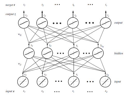
Neural networks are another method of function approximation. The training data consists of inputs \(\mathbf{x_i} \in \mathbb{R}^d_1\) and matching targets \(\mathbf{t_i} \in \mathbb{R}^d_2\). I will consider neural networks with a single hidden layer. In an arbitrarily large network with only one hidden layer, one can approximate any smooth function (see "Approximation by Superpositions of a Sigmoidal Function" - G. Cybenko (1989)).
In this section I will use superscript notation in brackets to index which layer, variables relate to. Layer 0 is the inputs, 1 is the hidden layer and 2 is the outputs. I write layer 2 (the last layer) as \(L\) incase I some day want to generalise this derivation to more hidden units.
Each unit in the network performs the following:
\begin{equation*} \text{The net activation of the j'th unit of layer l} = \mathrm{net}_j^{(l)}(\mathbf{x}) = \sum_{i=1}^dx_iw_{ji}^{(l)}+w_{j0}^{(l)} \end{equation*}The result of this is squashed by some non-linear function f(⋅)
\begin{equation*} \text{The output of the j'th unit of layer l} = y_j^{(l)}(\mathbf{x}) = f(\mathrm{net}_j^{(l)}(\mathbf{x})) \end{equation*}The sigmoid function is commonly used for this because it is what is used in biological neural networks and it relates to posterior probabilities.
Although the notation is slightly different, here is a picture of the kind of neural network I will be considering:
3.2.1 Backpropogation
The goal of backprogation is to learn the weights to use to achieve the lowest error.
We will use this error function:
\begin{equation*} J(\mathcal{W}) = \frac{1}{2}\sum_{i=1}^N||\mathbf{t}_i-\mathbf{y}_i^{(L)}||^2 \end{equation*}This is mean squared error for the i'th training sample (\(i=1,2,\dots,N\)). \(\mathcal{W}\) is the collection of all of the weights \(\{\mathbf{W}^{(l)}\}_{l=1}^L\). The factor of a half is just for algebraic convenience. As it is constant it does not effect the result.
As always, the objective is to minimise this error function with respect to these weights. Doing so with stochastic gradient decent requires the computation of
\begin{equation*} \Delta W_{pq}^{(l)} = - \eta \frac{\partial J}{\partial W_{pq}^{(l)}} \end{equation*}- The output layer
First lets consider doing this for the output layer (layer \(L\)):
\begin{align*} \frac{\partial J}{\partial W_{pq}^{(L)}} = \frac{\partial J}{\partial\mathrm{net}_p^{(L)}} \frac{\partial\mathrm{net}_p^{(L)}}{\partial W_{pq}^{(l)}} = -&\delta_p^{(L)}\frac{\partial\mathrm{net}_p^{(L)}}{\partial W_{pq}^{(l)}}\\ \text{Where }\quad &\delta_p^{(L)} := - \frac{\partial J}{\partial \mathrm{net}_p^{(L)}}\\ \therefore\: &\delta_p^{(L)} = -\underbrace{\frac{\partial J}{\partial y_p^{(L)}}}_\textit{Note 1} \overbrace{\frac{\partial y_p^{(L)}}{\partial \mathrm{net}_p^{(L)}}}^\textit{Note 2} = \underbrace{\left((\mathbf{t_{i}})_p - (\mathbf{y_{i}})_p^{(L)}\right)}_\text{Error at the output}\overbrace{f'(\mathrm{net}_p^{(L)})}^\text{Slope of non-linearity} \end{align*}Note 1: The partial differential of the error with respect to the output of the p'th node of the output layer
Note 2: The partial differential of the output of the p'th node of the output layer with respect to it's net activation
The other differential is trivial
\begin{equation*} \frac{\partial\mathrm{net}_p^{(L)}}{\partial W_{pq}^{(L)}} = (\mathbf{y_i})_{q}^{(L-1)} \quad =\quad \text{The output of the q'th unit of the previous layer} \end{equation*}So to summarise
\begin{equation*} \Delta W_{pq}^{(L)} = \eta\,\delta_p^{(L)}(\mathbf{y_i})_{q}^{(L-1)} \end{equation*} - The hidden layer
The hidden layer is layer \(l=L-1\)
\begin{equation*} \frac{\partial J}{\partial W_{pq}^{(l)}} = \frac{\partial J}{\partial (\mathbf{y_i})_p^{(l)}}\frac{\partial (\mathbf{y_i})_p^{(l)}}{\partial \mathrm{net}_p^{(l)}} \frac{\partial \mathrm{net}_p^{(l)}}{\partial W_{pq}^{(l)}} \end{equation*}Two of these are simple enough:
\begin{align*} \frac{\partial (\mathbf{y_i})_p^{(l)}}{\partial \mathrm{net}_p^{(l)}} &= f'(\mathrm{net}_p^{(l)}) \\ \frac{\partial \mathrm{net}_p^{(l)}}{\partial W_{pq}^{(l)}} &= (\mathbf{y_i})_{q}^{(l-1)} \end{align*}Note that layer 0 is the input layer and so for \(l=1\), \((\mathbf{y_i})_{q}^{(l-1)} = (\mathbf{x_i})_{q}\).
The remaining differential is more work:
\begin{align*} \frac{\partial J}{\partial (\mathbf{y_i})_p^{(l)}} &= \frac{\partial}{\partial (\mathbf{y_i})_p^{(l)}}\left( \frac{1}{2}\sum_{k=1}^c\left((\mathbf{t_i})_k - (\mathbf{y_i})_k^{(L)}\right)^2 \right) \\ &= -\sum_{k=1}^c\left((\mathbf{t_i})_k - (\mathbf{y_i})_k^{(L)}\right)\frac{\partial (\mathbf{y_i})_k^{(L)}}{\partial (\mathbf{y_i})_p^{(L-1)}} \\ &= -\sum_{k=1}^c\left((\mathbf{t_i})_k - (\mathbf{y_i})_k^{(L)}\right) \frac{\partial (\mathbf{y_i})_k^{(L)}}{\partial \mathrm{net}_k^{(L)}} \frac{\partial \mathrm{net}_k^{(L)}}{\partial (\mathbf{y_i})_p^{(L-1)}} \\ &= -\sum_{k=1}^c\left((\mathbf{t_i})_k - (\mathbf{y_i})_k^{(L)}\right) f'\left(\mathrm{net}_k^{(L)}\right)W_{kp}^{(L)} \\ &= -\sum_{k=1}^c \delta_k^{(L)} W_{kp}^{(L)} \\ \end{align*}So to summarise
\begin{equation*} \Delta W_{pq}^{(L-1)} = \eta\,f'(\mathrm{net}_p^{(L-1)})(\mathbf{y_i})_{q}^{(L-2)} \sum_{k=1}^c \delta_k^{(L)} W_{kp}^{(L)} \end{equation*}This means that the change in each hidden layer unit's weights is proportional to the error in each output it is connected to, scaled by this unit's weight on that output. This is why errors are said to propagate backwards through the network.
3.2.2 Speeding Up and Improving Performance
- Newton's Method can be used instead of gradient decent to converge quicker. However, this requires \(\mathcal{O}(N^2)\) storage and \(\mathcal{O}(N^3)\) computation.
- "Momentum" can be used to speed up learning in regions in which the gradient is small by adding a term relating to the gradient for the previous step to accelerate the decent down the gradient (by assuming that the gradient is in about the same direction as it was previously)
- As an alternative to newton's method, two subsequent gradient evaluations can be used to approximate local curvature, which may then be used in a second order method to achieve faster learning.
- Stop training early when cross-validation error begins to increase (indicating over fitting - high variance)
3.3 Classification
3.3.1 Bayesian Decision Theory
I will only consider gaussian distributed data. This is common because of the Central Limit Theorem. The aim is to learn the mean and co-variance for each class. Data can then be assigned to the most probable class.
We assume that we know the classes \(\omega_i, \, i=1,\dots,k\) and class probabilities \(P[\omega_i]\) a priori.
Training data tells us \(p(\mathbf{x} | \omega_i)\).
Formally, the decision rule is to find \(j\) such that
\begin{equation*} \max_j \left(P[\omega_j | \mathbf{x}]\right) \end{equation*}Using Bayes Theorem
\begin{equation*} P[\omega_j|\mathbf{x}] = \frac{p(\mathbf{x}|\omega_j)P[\omega_j]}{\sum_{i=1}^{k} p(\mathbf{x}|\omega_i) P[\omega_i]} \end{equation*}The denominator is constant with respect to \(j\) and so is unimportant for the maximum. Therefore the decision rule can be simplified to
\begin{equation*} \max_j \left( p(\mathbf{x}|\omega_j)P[\omega_j] \right) \end{equation*}The decision rule can be further simplified. For simplicity I will consider the two class case (\(k=2\)).
\begin{align*} p(\mathbf{x}|\omega_1)P[\omega_1] &\lessgtr p(\mathbf{x}|\omega_2)P[\omega_2] \\ \frac{1}{\sqrt{(2\pi)^p\mathrm{det}(\mathbf{C_1})}}\exp\left( -\frac{1}{2}(\mathbf{x} - \mathbf{m}_1)^T\mathbf{C_1}^{-1}(\mathbf{x} - \mathbf{m}_1) \right)P[\omega_1] &\lessgtr \frac{1}{\sqrt{(2\pi)^p\mathrm{det}(\mathbf{C_2})}}\exp\left( -\frac{1}{2}(\mathbf{x} - \mathbf{m}_2)^T\mathbf{C_2}^{-1}(\mathbf{x} - \mathbf{m}_2) \right)P[\omega_2] \end{align*}From this point we can get a few different classifiers, depending upon the assumptions we make. At first I will assume that the classes share a common co-variance matrix which shows no correlation of the variables (\(\mathbf{C} \propto \mathbf{I}\)) and that the prior probabilites of each class are equal.
\begin{align*} (\mathbf{x} - \mathbf{m}_1)^T\mathbf{C}^{-1}(\mathbf{x} - \mathbf{m}_1) &\lessgtr (\mathbf{x} - \mathbf{m}_2)^T\mathbf{C}^{-1}(\mathbf{x} - \mathbf{m}_2) \\ (\mathbf{x} - \mathbf{m}_1)^T(\mathbf{x} - \mathbf{m}_1) &\lessgtr (\mathbf{x} - \mathbf{m}_2)^T(\mathbf{x} - \mathbf{m}_2) \\ |\mathbf{x} - \mathbf{m}_1| &\lessgtr |\mathbf{x} - \mathbf{m_2}| \end{align*}This is a distance to mean classifier. To recap, to get to a distance to mean classifier, we had to assume that the variables were multivariate-gaussian distributed, with equal co-variance matrices with no correlation, equal prior class probabilities and distinct means.
A slightly more general classifier can be obtained by relaxing the assumptions that the co-variance matrices have no correlation and that the prior probabilities are equal.
\begin{align*} (\mathbf{x} - \mathbf{m}_1)^T\mathbf{C}^{-1}(\mathbf{x} - \mathbf{m}_1) + \log\left(\frac{P[\omega_1]}{P[\omega_2]}\right) &\lessgtr (\mathbf{x} - \mathbf{m}_2)^T\mathbf{C}^{-1}(\mathbf{x} - \mathbf{m}_2) \\ (\mathbf{x} - \mathbf{m}_1)^T\mathbf{C}^{-1}(\mathbf{x} - \mathbf{m}_1) -(\mathbf{x} - \mathbf{m}_2)^T\mathbf{C}^{-1}(\mathbf{x} - \mathbf{m}_2) + \log\left(\frac{P[\omega_1]}{P[\omega_2]}\right) &\lessgtr 0 \\ \mathbf{x}^T\mathbf{C}^{-1}\mathbf{x} -2\mathbf{m_1}^T\mathbf{C}^{-1}\mathbf{x} + \mathbf{m_1}^T\mathbf{C}^{-1}\mathbf{m_1} - \mathbf{x}^T\mathbf{C}^{-1}\mathbf{x} + 2\mathbf{m_2}^T\mathbf{C}^{-1}\mathbf{x} - \mathbf{m_2}^T\mathbf{C}^{-1}\mathbf{m_2} + \log\left(\frac{P[\omega_1]}{P[\omega_2]}\right) &\lessgtr 0 \\ 2(\mathbf{m_2} - \mathbf{m_1})^{T}\mathbf{C}^{-1}\mathbf{x} + \left[ \mathbf{m_1}^T\mathbf{C}^{-1}\mathbf{m_1} - \mathbf{m_2}^T\mathbf{C}^{-1}\mathbf{m_2} + \log\left(\frac{P[\omega_1]}{P[\omega_2]}\right) \right] &\lessgtr 0 \\ \end{align*}This is also a linear classifier because the assumption that the co-variance matrices are the same allowed the quadratic terms to cancel. This may also be considered as a distance to template classifier (as with the distance to mean classifier) except here we are using Mahalanobis distance instead of euclidean distance.
Relaxing that assumption (leaving only the assumption that the data are normally distributed) would lead to a quadratic classifier.
A similar application is to calculate the posterior probability of a gaussian distributed variable: (assuming that class 1 is not impossible)
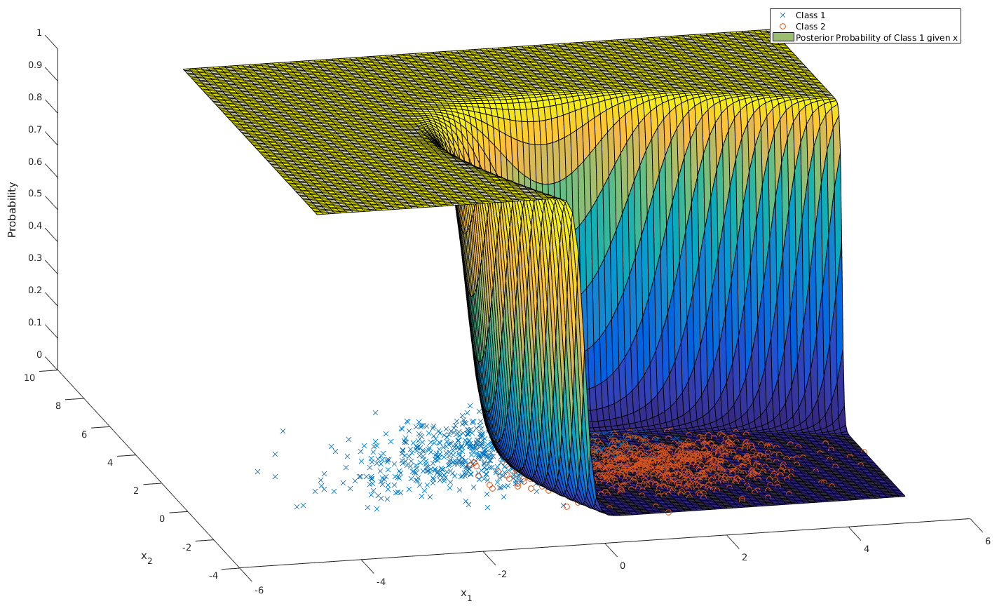
\begin{align*} P[\omega_1 | \mathbf{x}] &= \frac{p(\mathbf{x} | \omega_1)P[\omega_1]}{\sum_{i=1}^k p(\mathbf{x} | \omega_i)P[\omega_i]} \\ &= \frac{1}{1 + \sum_{i=2}^k \frac{p(\mathbf{x} | \omega_i)P[\omega_i]}{p(\mathbf{x} | \omega_1)P[\omega_1]}} \\ &= \frac{1}{1 + \sum_{i=2}^k \frac{P[\omega_i]\sqrt{\mathrm{det}(\mathbf{C}_1)}}{P[\omega_1]\sqrt{\mathrm{det}(\mathbf{C}_i)}}\exp\left[ (\mathbf{x} - \mathbf{m}_i)^T\mathbf{C_i}^{-1}(\mathbf{x} - \mathbf{m}_i) -(\mathbf{x} - \mathbf{m}_1)^T\mathbf{C_1}^{-1}(\mathbf{x} - \mathbf{m}_1) \right]} \\ \end{align*}As we saw previously, when the co-variances are equal, the exponential will be linear in \(\mathbf{x}\):
\begin{align*} P[\omega_1 | \mathbf{x}] &= \frac{1}{1 + \sum_{i=2}^k \frac{P[\omega_i]\sqrt{\mathrm{det}(\mathbf{C}_1)}}{P[\omega_1]\sqrt{\mathrm{det}(\mathbf{C}_i)}}\exp\left[\mathbf{w}^T\mathbf{x} + \mathbf{w}_0\right]} \\ \end{align*}For a two class problem, this is an obvious case of a sigmoidal function. For more classes or for a quadratic class boundary (distinct co-variance matrices), the plot still looks intuitively sigmoidal. For example, here is a 3D plot for two classes with different co-variance matrices:
3.3.2 Fisher Linear Discriminant Analysis
The idea behind fisher linear discriminant analysis is to project a higher dimensional problem which is hard to separate onto a lower dimensional surface which has chosen so as to maximise separability.
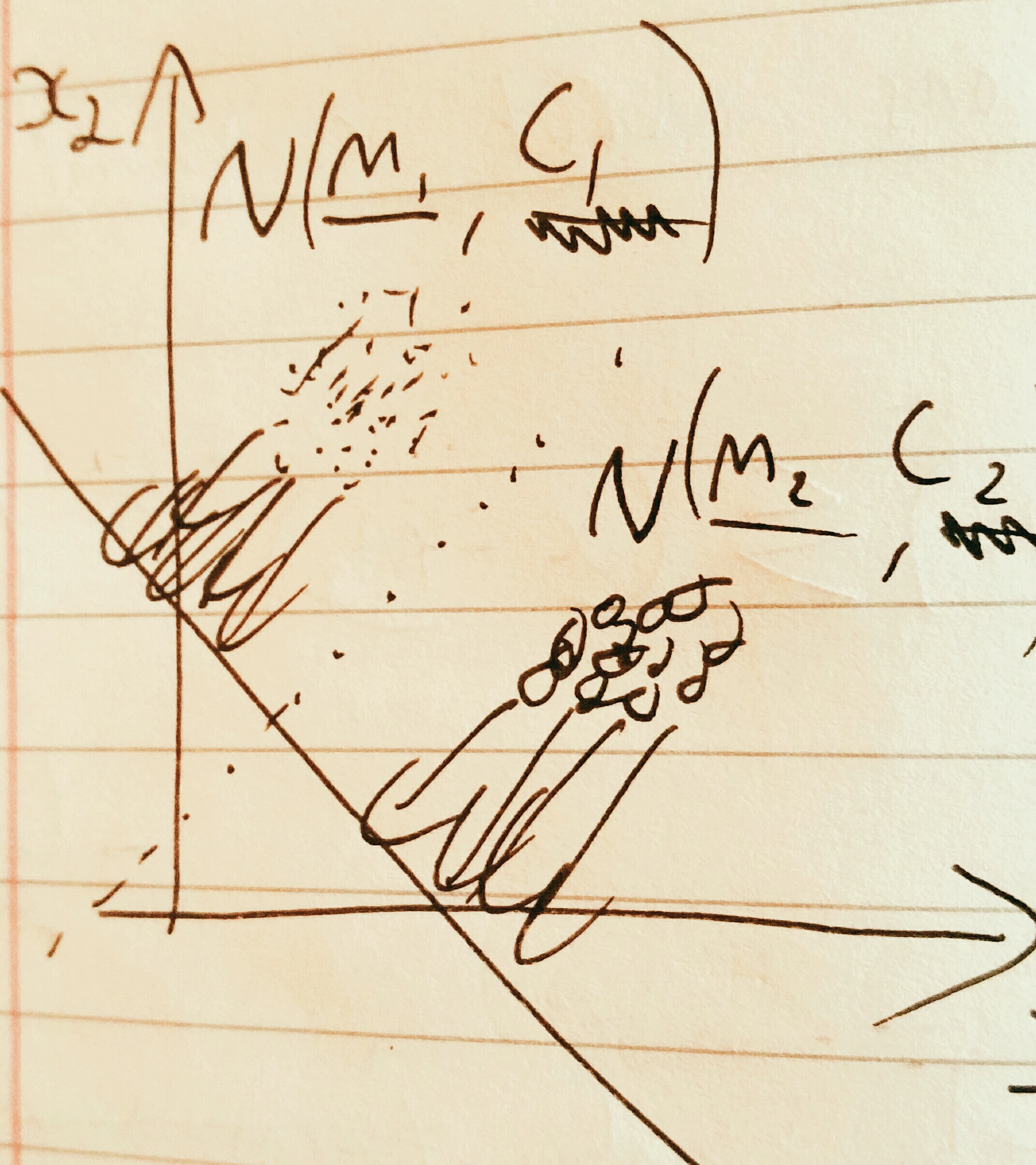
Considering the pictured problem of projecting a 2D problem onto 1D, the trick is to pick the gradient \(\mathbf{\omega} \in \mathbb{R}^d\) of the line so as to create maximal separability of classes. This can be captured by the fisher ratio: (recall that the scalar product projects one vector onto another)
\begin{equation*} J_F := \frac{(\mathbf{\omega}^T\mathbf{m}_1 - \mathbf{\omega}^T\mathbf{m}_2)^2}{\mathbf{\omega}^T\mathbf{C}_1\mathbf{\omega} + \mathbf{\omega}^T\mathbf{C}_2\mathbf{\omega}} \end{equation*}The fisher ratio can be thought of as the distance of the means divided by the variance on the line. Maximising this will make the points maximally separable because the means will have the greatest distance and the points will have as little spread about the mean as possible.
Another way of writing \(J_F\) is as a ratio of quadratic forms
\begin{align*} \mathbf{S_B} :=&\, (\mathbf{m}_1 - \mathbf{m}_2)(\mathbf{m}_1-\mathbf{m}_2)^T \\ \mathbf{S_W} :=&\, \mathbf{C}_1 + \mathbf{C}_2 \\ \therefore J_F =&\, \frac{\mathbf{\omega}^T\mathbf{S_B}\mathbf{\omega}}{\mathbf{\omega}^T\mathbf{S_W}\mathbf{\omega}} \end{align*}So to maximise \(J_F\):
\begin{align*} \frac{\partial J_F}{\partial \mathbf{\omega}} &= \mathbf{0} \\ &= \frac{2\mathbf{S_B\omega}(\mathbf{\omega}^T\mathbf{S_W\omega}) - 2\mathbf{S_W\omega}(\mathbf{\omega}^T\mathbf{S_B\omega})}{(\mathbf{\omega}^T\mathbf{S_W\omega})^2} \\ \end{align*}It is only the direction of \(\mathbf{\omega}\) which matters so we can just combine the scalars:
\begin{align*} \mathbf{S_B\omega}-\alpha_0\mathbf{S_W\omega} &= \mathbf{0} \\ \therefore \mathbf{S_W\omega} &= \alpha\mathbf{S_B\omega} \\ \end{align*}Note that
\begin{equation*} \mathbf{S_B\omega} = (\mathbf{m}_1 - \mathbf{m}_2)(\mathbf{m}_1-\mathbf{m}_2)^T\mathbf{\omega} = (\mathbf{m}_1 - \mathbf{m}_2)\alpha_1 \end{equation*}And so points in the same way as \(\mathbf{m}_1 - \mathbf{m}_2\). From this we have an equation for \(\omega\)
\begin{equation*} \mathbf{\omega} = \alpha_2(\mathbf{C_1} + \mathbf{C_2})^{-1}(\mathbf{m}_1 - \mathbf{m}_2) \end{equation*}Once projected onto this line, data should be more easily separable using Bayesian Decision Theory.
3.3.3 Perceptron
Perceptron follows a similar process to linear regression except the output is discrete: \(f \: : \: \mathbb{R}^p \to \{1, -1\}\). Our model is
\begin{equation*} f(\mathbf{x}) := \begin{cases} +1 & \mathbf{w}^T\mathbf{x} + w_0 \geq 0 \\ -1 & \mathbf{w}^T\mathbf{x} + w_0 < 0 \end{cases} \end{equation*}Note that the output when the model gives zero is arbitrary.
As with linear regression we will use \(\mathbf{w}^T\mathbf{x} + w_0 \equiv \mathbf{y}^T\mathbf{a}\).
The intuitive choice for an error function is to count the number of missclassifications. However, this would create an function which steps discretely (looking like stairs). This is piecewise constant and so cannot be differentiated and so is hard to minimise. Instead we will use the the sum of function outputs across the set of unclassified items \(\mathcal{U}\).
\begin{equation*} E = -\sum_{\mathbb{y}_n \in \mathcal{U}}\mathbf{y}_n^T\mathbf{a} \end{equation*}This may then be minimised using stochastic gradient decent. First the derivative:
\begin{equation*} \frac{\partial E}{\partial \mathbf{a}} = -\sum_{\mathbb{y}_n \in \mathcal{U}}\mathbf{y}_n \end{equation*}Therefore, using randomly chosen \(\mathbf{y}_n\) we can update like this
\begin{equation*} \mathbf{a}^{(k+1)} = \mathbf{a}^{(k)} + \mathbf{y}_n \end{equation*}3.3.4 Support Vector Machines
Here we will only consider a brief introduction to support vector machines in which data are linearly separable.
The problem with perceptron classification is that it makes no distinction between decision boundaries which only work for the training data and decision boundaries which generalise well to unseen data. The idea in support vector machines is to maximise the margin between the decision boundary and the edges of the classes to be separated so that the likelihood of unseen data being found on the wrong side of the decision boundary is minimised. Intuitively this is like trying to draw the thickest decision line as possible.
Notation:
\begin{align*} \text{Decision boundary hyperplane:} &\quad \mathbf{w}^T\mathbf{x}+b=0 \\ \text{Data:} &\quad \mathcal{D} = \{\mathbf{x}_n, y_n\}^N_{n=1}, \quad \mathbf{x}_n\in\mathbb{R}^d,\quad y_n \in \{-1, +1\} \\ \text{Learning problem:} &\quad y_n(\mathbf{w}^T\mathbf{x}+b)\geq 1 \quad \forall n=1,2,\dots,N \end{align*}Assume that the decision boundary defined by \((\mathbf{w}, b)\) separates the data. Therefore the following can be derived:
\begin{align*} \left(\text{Width of margin}\right) &= \left(\text{Distance from the decision boundary to the closest point in class -1}\right) + \left(\text{Distance from the decision boundary to the closest point in class +1}\right) \\ &= \min_{\mathbf{x}_n:\,y_n=-1}\left(\frac{|\mathbf{w}^T\mathbf{x}_n+b|}{||\mathbf{w}||}\right) + \min_{\mathbf{x}_n:\,y_n=+1}\left(\frac{|\mathbf{w}^T\mathbf{x}_n+b|}{||\mathbf{w}||}\right) \\ &= \frac{1}{||\mathbf{w}||}\left( \min_{\mathbf{x}_n:\,y_n=-1}\left(|\mathbf{w}^T\mathbf{x}_n+b|\right) + \min_{\mathbf{x}_n:\,y_n=-1}\left(|\mathbf{w}^T\mathbf{x}_n+b|\right) \right) \\ &= \frac{1}{||\mathbf{w}||}\left( k_1 + k_2 \right) \end{align*}\(k_1\) and \(k_2\) are influenced more by the particular training data than anything else and their variation is not important because with a constant dataset, changing \(\mathbf{w}\) or \(b\) will not change the result of \(k_1 + k_2\) (because going closer to one class means going further from another). As we have assumed that the learning problem is solved, \(k_1 + k_2\) cannot be smaller than \(2\) for any data (each \(k_n\) must be at least 1 for the learning condition to hold).
So to solve the initial problem, we want to find the \(\mathbf{w}\) which maximises this margin width, under the constraints that all data points are correctly classified according to the learning problem:
\begin{equation*} \max_\mathbf{w}\left(\frac{1}{||\mathbf{w}||}\right) \quad \text{subject to} \quad y_n(\mathbf{w}^T\mathbf{x}_n+b)\geq 1 \quad \forall n \end{equation*}This function is not a nice shape for optimisation so we will instead solve the equivalent problem
\begin{equation*} \min_\mathbf{w}\left(||\mathbf{w}||^2\right) \quad \text{subject to} \quad y_n(\mathbf{w}^T\mathbf{x}_n+b)\geq 1 \quad \forall n \end{equation*}As this is quadratic, it will behave well. Writing this as a lagrangian is the following:
\begin{equation*} \mathcal{L}(\mathbf{w}, b, \mathbf{\lambda}) := ||\mathbf{w}||^2 - \sum_{n=1}^N\lambda_n(y_n(\mathbf{w}^T\mathbf{x}_n+b)-1), \, \lambda_n \geq 0 \end{equation*}As always with these problems we set \(\mathbf{\nabla}\mathcal{L} = \mathbf{0}\).
\begin{align*} \frac{\partial\mathcal{L}}{\partial b} =0 &\implies \sum_{n=1}^N\lambda_ny_n=0 \\ \frac{\partial\mathcal{L}}{\partial \mathbf{w}} = 0 &\implies \mathbf{w} = \sum_{n=1}^N\lambda_ny_n\mathbf{x}_n \end{align*}This leads to the following quadratic programming problem, which can be solved numerically.
\begin{equation*} \min_\mathbf{\lambda}\left(\sum_{i=1}^N\sum_{j=1}^N\lambda_i\lambda_jy_iy_j\mathbf{x}_i^T\mathbf{x_j}-\sum_{k=1}^N\lambda_k\right) \quad \text{subject to} \quad \lambda_n \geq 0 \quad \text{and} \quad \sum_{n=1}^N\lambda_ny_n=0 \end{equation*}Finally, the bias term can be found using the support vectors \(\mathbf{x}_n\)
\begin{align*} y_n\left(\mathbf{w}^T\mathbf{x}_n + b\right) = 1 \\ y_n^2\left(\mathbf{w}^T\mathbf{x}_n + b\right) = y_n \\ 1\left(\mathbf{w}^T\mathbf{x}_n + b\right) = y_n \\ \therefore b = y_n -\mathbf{w}^T\mathbf{x}_n \end{align*}In practice, an average will be taken over all support vectors
\begin{equation*} b = \frac{1}{N}\sum_{n=1}^N\left(y_n -\mathbf{w}^T\mathbf{x}_n\right) \end{equation*}3.4 Estimation
I will not discuss Baysean estimation.
Estimation is about working out the parameters used in probability distributions. When looking at a datum we consider how probable (likely) it is. We can consider the probability as parameterised by the things we are trying to estimate. For example, the probability of gaussian-distributed data is parameterised by it's mean and variance (we will not consider multivariate parameter estimation). In notation, for data \(x\) parameterised by \(\mathbf{\theta}\); we say that the likelihood is \(p(x|\mathbf{\theta})\).
For a dataset \(\mathbb{D} = \{x_i\}, \: i = 1, 2, \dots, N\), we assume that the events are independent:
\begin{equation*} p(\mathbb{D}|\mathbf{\theta}) = \prod_{x_i \in \mathbb{D}} p(x_i|\mathbf{\theta}) \end{equation*}To find the most likely parameters, we will maximise the likelihood of the whole dataset with respect to \(\mathbf{\theta}\). To do this we will use the logarithm of the likelihood because this turns the product into a sum: therefore making the differentiation easier.
\begin{equation*} l(\mathbf{\theta}) := \ln\left( p(\mathbb{D} | \mathbf{\theta}) \right) \end{equation*}So we are trying to work out \(\hat{\mathbf{\theta}} = \mathrm{arg} \, \max_{\mathbf{\theta}} \, l(\mathbf{\theta})\).
As always, this means differentiating and setting it equal to zero:
\begin{equation*} \mathbf{\nabla_\theta}l = \mathbf{\nabla_\theta}\left( \sum_{x_i \in \mathbb{D}}\ln\left[ p(x_i|\mathbf{\theta}) \right] \right) = \mathbf{0} \end{equation*}3.4.1 Example - Univariate Gaussian Data
So substituting in using \(\theta_1 = m\) and \(\theta_2 = \sigma^2\)
\begin{equation*} \mathbf{\nabla_\theta}l = \mathbf{\nabla_\theta}\left( \sum_{x_i \in \mathbb{D}}\left[ \frac{1}{2}\ln(2\pi\theta_2)-\frac{1}{2\theta_2}(x_i-\theta_1)^2 \right]\right) = \mathbf{0} \end{equation*}Therefore
\begin{equation*} \begin{pmatrix} \sum_{x_i \in \mathbb{D}}\frac{1}{\hat{\theta_2}}(x_i - \hat{\theta_1}) \\ \sum_{x_i \in \mathbb{D}}\left[ \frac{-1}{2\hat{\theta_2}} + \frac{1}{\hat{\theta_2}^2}\left( x_j - \hat{\theta_1} \right)^2\right] \\ \end{pmatrix} = \begin{pmatrix} 0 \\ 0 \end{pmatrix} \end{equation*}After some algebra
\begin{align*} \hat{m} = \hat{\theta_1} &= \frac{1}{N}\sum_{x_i \in \mathbb{D}}x_i \\ \hat{\sigma^2} = \hat{\theta_2} &= \frac{1}{N}\sum_{x_i \in \mathbb{D}}\left(x_i - \hat{m}\right)^2 \end{align*}4 Unsupervised Learning
4.1 Principle Component Analysis
Principle component analysis reduces the dimensionality of data. This can be useful for compression.
Let there be N items of data \(\mathbf{x}_n \in \mathbb{R}^d\) with mean \(\mathbf{m}\) and covariance \(\mathbf{C}\). We will project the data into the direction \(\mathbf{u}\). To maximise the amount of data represented in the projection, we want the highest variance possible in the projection. To optimise this we need a constraint on \(\mathbf{u}\) as the problem does not specify it's magnitude. As the magnitude of \(\mathbf{u}\) is unimportant, I will set it to 1.
Therefore the optimisation problem can be set up as follows:
\begin{equation*} \max_\mathbf{u} \: \mathbf{u}^T\mathbf{C}\mathbf{u} \quad \mathrm{subject\: to} \: \mathbf{u}\cdot\mathbf{u} = 1 \end{equation*}As a lagrange multiplier problem
\begin{align*} \mathbf{\nabla}\mathcal{L} &= \mathbf{\nabla}\left\{\mathbf{u}^T\mathbf{Cu} - \lambda(\mathbf{u}^T\mathbf{u} - 1)\right\} = \mathbf{0} \\ \therefore \frac{\partial \mathcal{L}}{\partial \mathbf{u}} &= 2\mathbf{Cu}-2\lambda(\mathbf{u}-1) = \mathbf{0} \\ \therefore \mathbf{Cu} &= \lambda\mathbf{u} \end{align*}So the solutions to the principle component values problem are the eigen vectors of \(\mathbf{C}\).
4.2 Clustering
4.2.1 Expectation Maximisation (EM)
Assuming we have some prior knowledge of the number of classes we expect, \(K\), we would intuitively expect data to be in a \(K\)-modal distribution (as usual we are using the normal distribution):
\begin{equation*} p(\mathbf{x}) = \sum_{k=1}^K\pi_k\mathcal{N}(\mathbf{m}_k, \mathbf{C}_k) \end{equation*}The \(\pi_k\) parameters can be thought of as the prior probabilities of each class (mode).
The aim of this algorithm is to find \(z_{nk}\): associating nth data to kth class. This can be decided by comparing the probabilities of data belonging to each class.
For parameter estimation we have to estimate \(\pi_k\), \(\mathbf{m}_k\) and \(\mathbf{C}_k\). The algebra for this is hard. Ultimately, \(\pi_k\), \(\mathbf{m}_k\) and \(\mathbf{C}_k\) become parameterised by \(q_{nk}\), which can be interpreted as the probability that a point \(n\) is in cluster \(k\).
A useful example is the result for \(\mathbf{m}_k\):
\begin{equation*} \mathbf{m}_k = \frac{\sum_{n=1}^Nq_{nk}\mathbf{x}_n}{\sum_{n=1}^Nq_{nk}} \end{equation*}Here the contribution of point \(\mathbf{x}_n\) to the mean of a cluster is weighted by the probability that the point is in that cluster.
The formula for \(q_{nk}\) is also worth commenting upon
\begin{equation*} q_{nk} = \frac{\pi_kp(\mathbf{x}_n|\mathbf{m}_k, \mathbf{C}_k)}{\sum_{j=1}^K\pi_jp(\mathbf{x}_n|\mathbf{m}_j, \mathbf{C}_j)} \end{equation*}This is interesting because it is Bayes formula for \(p(z_{nk}=1|\mathbf{x}_n, \pi_k, \mathbf{m}_k, \mathbf{C}_k)\).
As the estimated parameters and \(q_{nk}\) depend upon each-other, EM must be solved itteritively. One way to do this is to pick \(q_{nk}\) by considering the distance to means and then to use these to compute the other parameters.
4.2.2 K-Means
The K-Means algorithm on input \(\mathbf{X} = \{\mathbf{x}_n\}_{n=1}^N,\:K\) outputs a vector of mode centres \(\mathbf{C}\) and \(\mathrm{Idx}\), a vector containing the class assigned to each data point.
repeat
    assign n'th sample to the nearest centre
    recompute centres by averaging all the points assigned to them
until no change in the centres
K-means can be derived from EM by setting qnk to 1 for only the largest qnk over each k and the other cells to 0. Therefore the re-estimation of \(\mathbf{m}_k\) and \(\mathbf{C}_k\) become maximum likelihood estimates. K-means should be thouht of as like EM except data are either in one class or another: nothing probabilistic. Also, standard k-means does not use covariance matrices.